8 STL decomposition

The three components (Fig. 8.1) capture different aspects of the total PM_2.5 timeseries. Long-term variation (over years) is found in trend, which in the case shown, is a slight decrease over 2015. Year-to-year changes in PM_2.5 are typically low (less than 1µg/m³) and thus trend does not typically vary significantly. The seasonal component, in contrast, represents regular fluctuations in the timeseries. Here the fluctuations tend to depend on the time of year and the seasonal component is similar (though not exactly the same) for each year. In this example, the higher seasonal PM_2.5 during May to October is a reflection of the regular dry season bushfires in the Northern Territory.

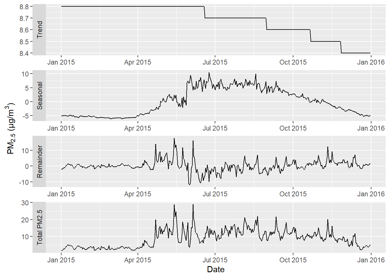
Figure 8.1: STL components and total PM2.5 concentration for a pixel in Darwin (NT) for the year 2015.

The seasonal pattern can vary greatly from one location to another, depending on climate and the surrounding environment. While in Darwin, bushfires are expected in the dry season (winter months), south-eastern Australia typically experiences bushfires in the summer months and would see peaks of seasonal PM_2.5 through December to February, as in Campbelltown (NSW). High seasonal PM_2.5 is also not necessarily indicative of bushfires. For instance, Launceston (Tasmania) experiences high seasonal PM_2.5 through winter months, not due to bushfires but rather domestic wood heater smoke (Fig. 8.2).

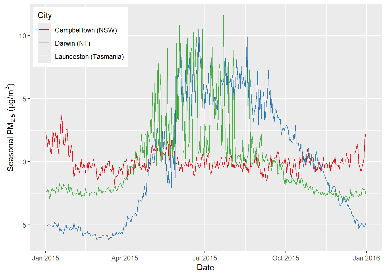
Figure 8.2: Comparison of seasonal components for locations of contrasting environment and climate around Australia - Darwin (NT), Campbelltown (NSW) and Launceston (Tasmania).

Together, the trend and seasonal components are a expectation of the PM_2.5 concentration given the long-term and seasonal variations. The remainder is therefore represents the fluctuations around the expected value.

Figure 8.3: Cumulative addition of STL components to total PM2.5 concentration for pixel in Darwin (NT) for the year 2015.

The three STL components sum to the total PM_2.5, illustrated in Figure 8.3. Note that both the seasonal and remainder components are often negative - the seasonal component captures regular variations around the long-term trend and the remainder component the fluctuations around ‘expectation’, trend + seasonal.

8.1 Quantification of bushfire-specific PM_2.5

It is important to note that the STL alone does not indicate the presence of bushfire smoke-related PM_2.5. Additional information such as the flags are required to classify days as being bushfire-affected or not.

The STL decomposition does allow a degree of quantification of bushfire-specific PM_2.5 once those bushfire-affected days are identified. Different approaches are possible and the best option will depend on the study question.

Taking, for instance, the Darwin example above (Fig. 8.1), the seasonal component includes the expected regular bushfire-related PM_2.5 during the dry season. Increased remainder indicates a worse-than-usual bushfire-affected day (higher PM_2.5) and conversely decreased remainder shows this day was less affected than usual or not affected at all.

Thus the difference between remainder and seasonal + trend (expectation) for a bushfire-affected day (assuming bushfires to be the dominant source of PM_2.5) is only a partial representation of the full PM_2.5 due to bushfires. This may be a reasonable measure if the study is concerned with exceptionally poor air quality due to bushfire events of greater than usual severity.

An alternative approach is to identify a bushfire-affected day then assume all PM_2.5 above some background level to be attributable to bushfire smoke. This is a more inclusive approach but could overestimate if there are other significant sources of PM_2.5 on those days. Furthermore, what is regarded as background is not clearly defined (e.g. could be the trend value, an arbitrary set value, or a statistical threshold value such as the annual mean). Again, this should be considered with respect to the study question.